其他專案 · Selected Work · 2025

Homography Estimation

3D Computer Vision 課程作業：從兩張視角不同的照片中，用 SIFT 找特徵點配對，挑出分布分散的優質點，透過 Normalized DLT + RANSAC 手刻算出 Homography 矩陣，再用雙線性插值把一張圖片 warp 成另一張圖片的視角。

電腦視覺 / 幾何轉換 3D Computer Vision · HW1 2025

要解決的問題

這是「3D Computer Vision」課程的作業：給定同一個平面（磁磚地板）在不同視角拍攝的兩張照片，求出一個 3×3 Homography 矩陣 H，能把其中一張圖片的每個像素座標，對應到另一張圖片中同一個平面點的座標。作業要求整條 pipeline 都要自己刻：特徵點取樣策略、Normalized DLT、RANSAC、以及最後用 H 做 image warping，不能直接呼叫 cv2.findHomography。

流程 Outline

取得待轉換圖片與兩張目標圖片，做 SIFT 特徵點配對
從配對結果中取優質的 k 個點做 Homography 估計（k ≥ 4）
把點歸一化（Normalize），統一資料尺度，避免特徵點座標大小不一影響數值穩定性
做 Normalized DLT，並用 RANSAC 迭代取誤差最小的解，算出 Homography 矩陣
計算 projection error 驗證結果
Warping：把來源圖片透過 H 矩陣轉換成目標圖片視角

SIFT 特徵配對

SIFT（Scale-Invariant Feature Transform）在圖片中找出不會因縮放、旋轉、亮度變化而失效的穩定特徵點：先用高斯金字塔與 DoG 在不同尺度找局部極值當候選關鍵點，過濾掉低對比度與邊緣上的不穩定點，再依周圍梯度方向給每個點一個主方向，最後用 128 維梯度方向直方圖當描述子。兩張圖片的描述子之間用 BFMatcher 做 k=2 的 knnMatch，再用 Lowe's ratio test（次佳距離的 0.75 倍）篩掉容易錯配的模糊點。

def get_sift_correspondences(img1, img2):
    sift = cv.SIFT_create()
    kp1, des1 = sift.detectAndCompute(img1, None)
    kp2, des2 = sift.detectAndCompute(img2, None)

    matcher = cv.BFMatcher()
    matches = matcher.knnMatch(des1, des2, k=2)
    good_matches = []
    for m, n in matches:
        if m.distance < 0.75 * n.distance:   # Lowe's ratio test
            good_matches.append(m)

    good_matches = sorted(good_matches, key=lambda x: x.distance)
    points1 = np.array([kp1[m.queryIdx].pt for m in good_matches])
    points2 = np.array([kp2[m.trainIdx].pt for m in good_matches])
    return points1, points2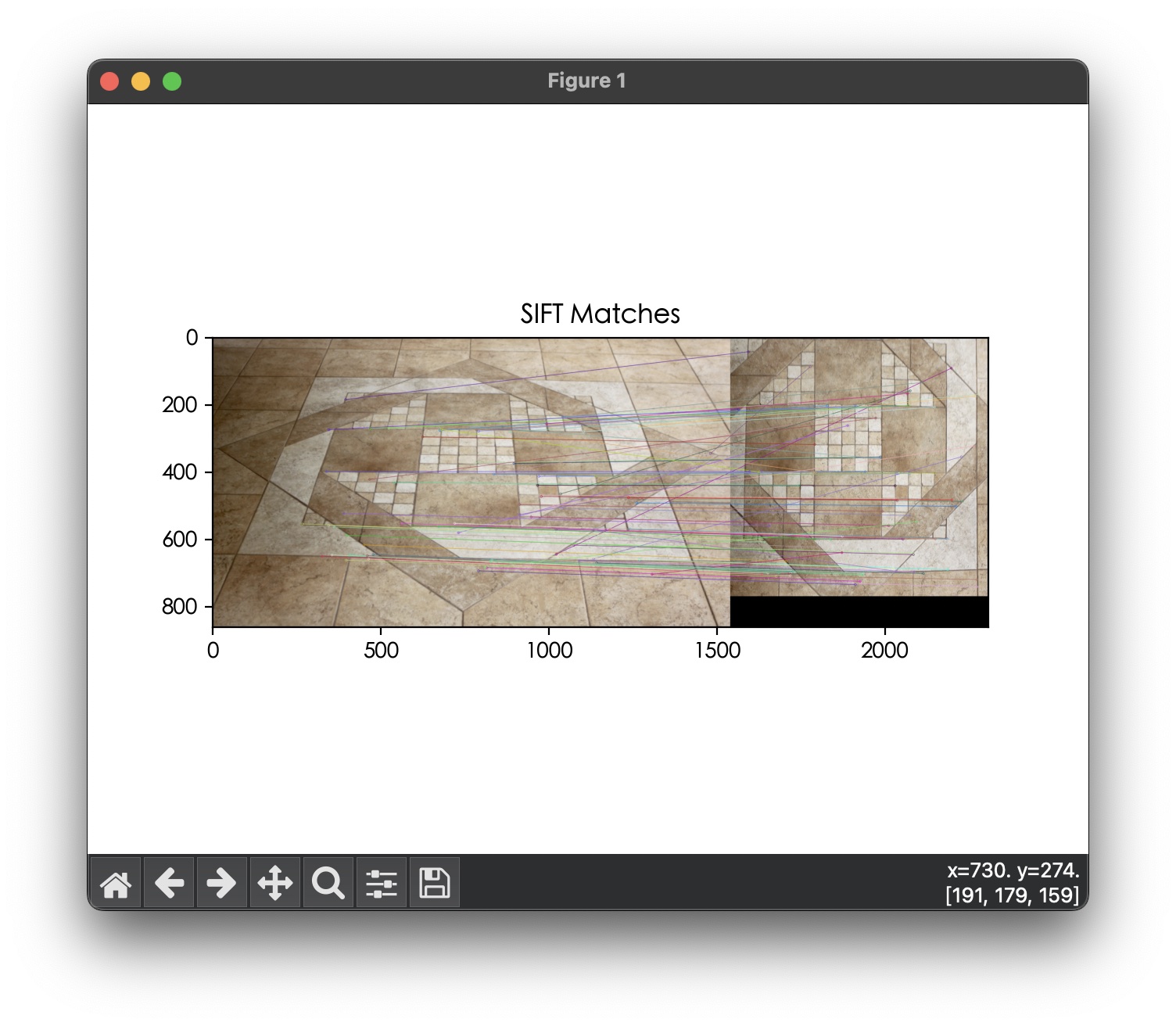

get_sift_correspondences() — SIFT 偵測 + BFMatcher 配對 + ratio test 篩選

SIFT Matches 視覺化：兩張磁磚地板照片並排，之間用彩色線條連接對應的特徵點，線條大致沿著透視方向分佈，顯示 SIFT 找到的匹配點多數落在正確的對應位置上。

SIFT 特徵配對結果：兩張圖片間的對應點以彩色線條連接

k_point_sample()：象限分散取樣

優質點不能只看配對距離，還要考慮空間分布：參考點越分散，算出來的 Homography 對整張圖片的還原效果越好。做法是先把圖片切成四個象限，每個象限依序取距離最小（最優質）的點，直到湊滿 k 個；若某象限找不到剩餘的優質點，就用隨機點補齊，確保 k 個點不會全部擠在同一區域。

def k_point_sample(points1, points2, img1, k):
    amount = 40
    points1, points2 = points1[:amount], points2[:amount]

    center_x, center_y = img1.shape[1] / 2, img1.shape[0] / 2
    quadrant1 = (points1[:, 0] > center_x) & (points1[:, 1] > center_y)
    quadrant2 = (points1[:, 0] < center_x) & (points1[:, 1] > center_y)
    quadrant3 = (points1[:, 0] < center_x) & (points1[:, 1] < center_y)
    quadrant4 = (points1[:, 0] > center_x) & (points1[:, 1] < center_y)
    quadrants = [quadrant1, quadrant2, quadrant3, quadrant4]

    selected_points1, selected_points2 = [], []
    while len(selected_points1) < k:
        for q in quadrants:
            found = False
            for i, flag in enumerate(q):
                if flag:
                    selected_points1.append(points1[i])
                    selected_points2.append(points2[i])
                    q[i] = False
                    found = True
                    break
            if not found:                      # 該象限沒有剩餘優質點，補隨機點
                randint = np.random.randint(0, len(points1))
                selected_points1.append(points1[randint])
                selected_points2.append(points2[randint])

    return np.array(selected_points1), np.array(selected_points2)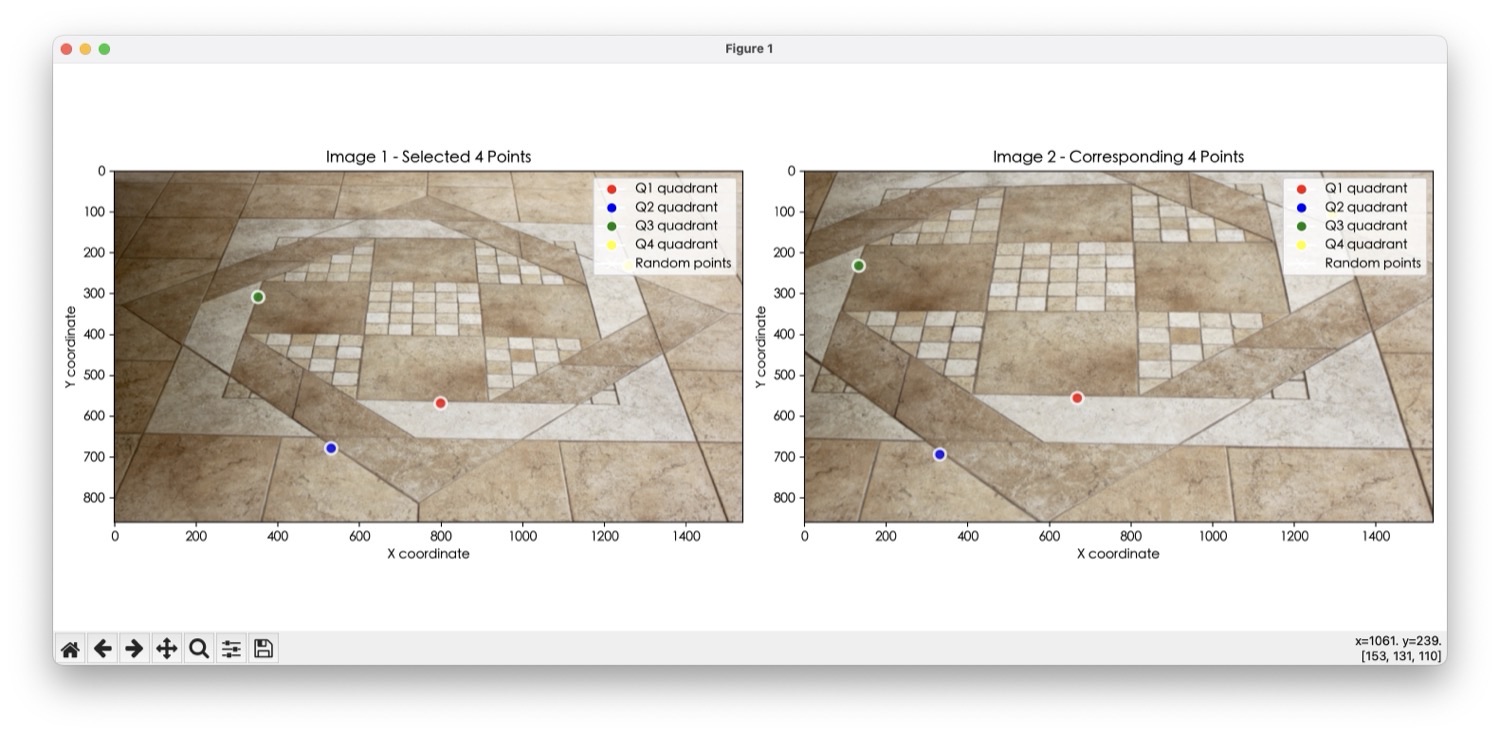

k_point_sample() — 四象限輪流取優質點，取不到就隨機補齊

兩張並排的散點圖，分別標題為 Image 1 - Selected 4 Points 與 Image 2 - Corresponding 4 Points，各用紅、藍、綠、黃四種顏色標出 Q1 到 Q4 象限選出的四個對應點，兩張圖上同色的點位置互相對應。

k=4 時的取樣結果：四個象限（紅、藍、綠、黃）各取一點，兩張圖上的對應點顏色一致

計算 Homography 矩陣

Homography 轉換的核心公式是 x' = Hx：原始圖片的一個二維點 [x, y] 先轉成齊次座標 [x, y, 1]，乘上 3×3 的 H 矩陣後得到目標座標系中的位置。當 k=4 時，四個點都是 SIFT 排序後最優質的點，不做 RANSAC 效果也不錯；但當 k 變大（例如 k=20）時，取樣進來的點難免混入劣質配對，這時就必須用 RANSAC 隨機取樣、迭代找出誤差最小的 4 點組合，再用這組 inliers 重新算一次最終的 H。

def homography_estimation(points1, points2):
    threshold, max_iter = 3.0, 2000
    n = points1.shape[0]
    best_H, best_inliers, max_inliers = None, None, 0

    for _ in range(max_iter):
        if n < 4: continue
        sample_indices = np.random.choice(n, 4, replace=False)
        try:
            H_candidate = compute_homography(points1[sample_indices], points2[sample_indices])
        except:
            continue

        pts1_h = np.hstack([points1, np.ones((n, 1))])
        projected = (H_candidate @ pts1_h.T).T
        projected /= projected[:, 2:3]               # 齊次座標歸一化
        dists = np.linalg.norm(projected[:, :2] - points2, axis=1)

        inliers = dists < threshold
        if np.sum(inliers) > max_inliers:
            max_inliers = np.sum(inliers)
            best_H, best_inliers = H_candidate, inliers

    if best_inliers is not None and np.sum(best_inliers) >= 4:
        best_H = compute_homography(points1[best_inliers], points2[best_inliers])  # 用全部 inliers 重估
    return best_H

homography_estimation() — RANSAC：隨機取 4 點 → 算 H → 數 inliers → 保留最佳解 → 用 inliers 重估

底層的 compute_homography() 則是標準的 Normalized DLT：先各自把兩組點平移縮放到「平均中心在原點、平均距離 √2」，用歸一化後的座標組出線性方程組 A，SVD 分解取最小奇異值對應的向量重塑成 3×3 矩陣，最後再用歸一化矩陣的反矩陣把 H 反歸一化（denormalize）回原始座標系。歸一化這一步很關鍵——像素座標數值範圍可能到幾千，直接做 DLT 容易讓 SVD 數值不穩定。

def normalize_points(points):
    """平移縮放到：平均中心在 (0,0)，平均距離 = sqrt(2)"""
    n = points.shape[0]
    mean = np.mean(points, axis=0)
    dist = np.sqrt(np.sum((points - mean) ** 2, axis=1))
    scale = np.sqrt(2) / np.mean(dist)

    T = np.array([[scale, 0, -scale * mean[0]],
                  [0, scale, -scale * mean[1]],
                  [0, 0, 1]])
    pts_h = np.hstack([points, np.ones((n, 1))])
    return (T @ pts_h.T).T[:, :2], T

def compute_homography(points1, points2):
    """Normalize -> DLT -> Denormalize"""
    pts1_norm, T1 = normalize_points(points1)
    pts2_norm, T2 = normalize_points(points2)

    A = []
    for (x1, y1), (x2, y2) in zip(pts1_norm, pts2_norm):
        A.append([-x1, -y1, -1, 0, 0, 0, x1*x2, y1*x2, x2])
        A.append([0, 0, 0, -x1, -y1, -1, x1*y2, y1*y2, y2])
    A = np.array(A)

    _, _, Vt = np.linalg.svd(A)
    Hn = Vt[-1].reshape(3, 3)

    H = np.linalg.inv(T2) @ Hn @ T1                  # denormalize
    return H / H[2, 2]

normalize_points() + compute_homography() — Normalized DLT 的完整流程

Homography Warping

目標是把來源圖片變成目標圖片的視角：先建一張跟目標圖片一樣大的空白畫布， 反向掃描——對目標畫布上的每個座標點，用 H 的反矩陣 算回它在來源圖片上對應的位置，再用雙線性插值取出該位置附近四個像素的加權平均當作最終顏色。用反向映射（而不是正向把來源每個像素往前推）可以避免目標圖片上出現沒有被填到值的空洞。

def homography_warping(img1, img2, H):
    h, w = img2.shape[0], img2.shape[1]
    img1_wrap = np.zeros_like(img2)
    H_inv = np.linalg.inv(H)                          # 目標 → 來源 的反向映射

    for y in range(h):
        for x in range(w):
            src_pt = H_inv @ np.array([x, y, 1])
            src_pt /= src_pt[2]
            src_x, src_y = src_pt[0], src_pt[1]

            if 0 <= src_x < img1.shape[1]-1 and 0 <= src_y < img1.shape[0]-1:
                x0, y0 = int(np.floor(src_x)), int(np.floor(src_y))
                x1, y1 = x0 + 1, y0 + 1
                dx, dy = src_x - x0, src_y - y0
                val = (img1[y0, x0] * (1-dx) * (1-dy) +
                       img1[y0, x1] * dx * (1-dy) +
                       img1[y1, x0] * (1-dx) * dy +
                       img1[y1, x1] * dx * dy)          # 雙線性插值
                img1_wrap[y, x] = val

    return img1_wrap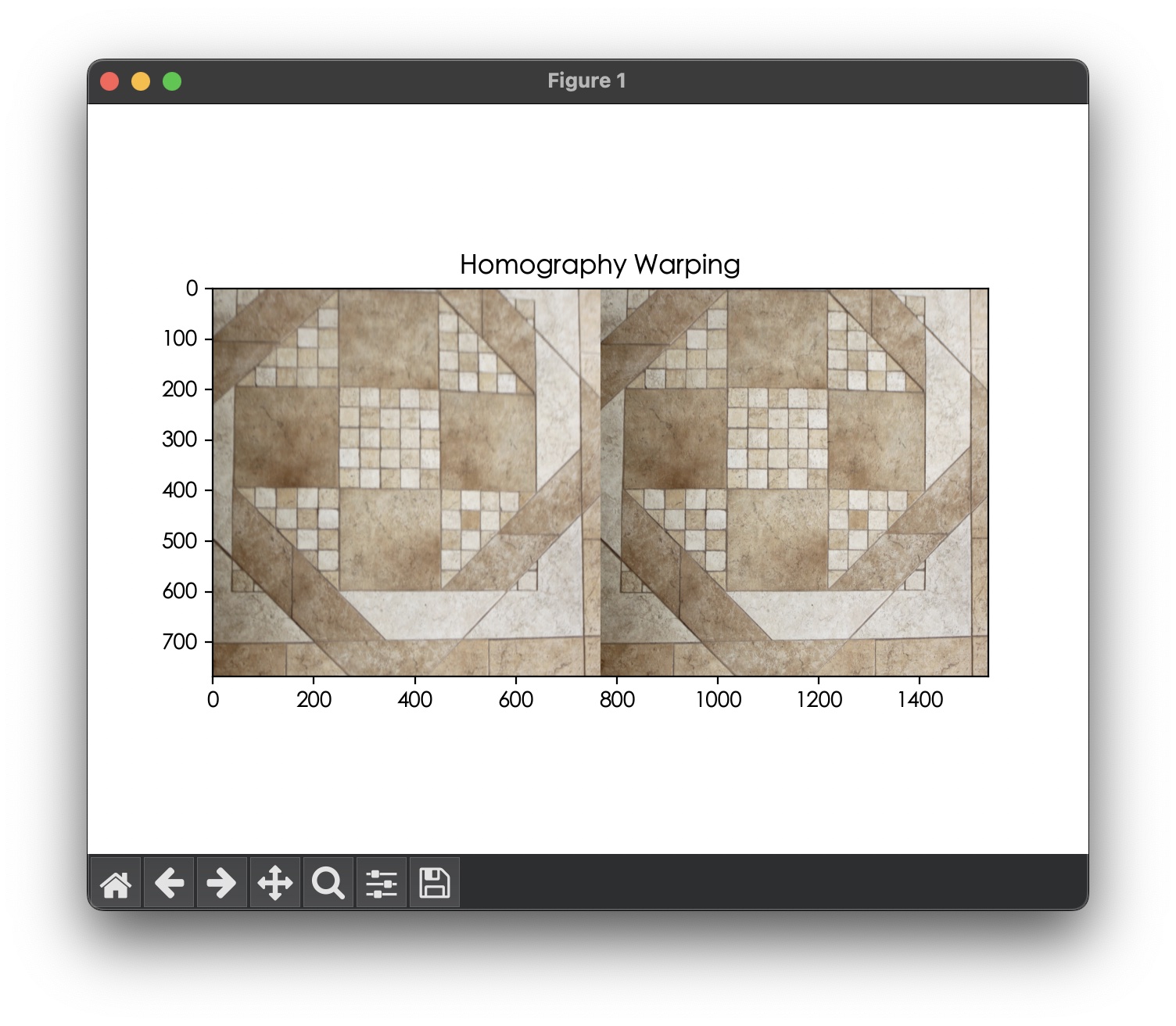

homography_warping() — 反向映射 + 雙線性插值，避免目標圖片出現空洞

Homography Warping 結果：左右並排兩張磁磚地板圖片，圖案、透視角度與拼接紋理幾乎完全一致，顯示來源圖片經過 H 矩陣轉換後成功還原成目標圖片的視角。

Warping 結果：左圖是用計算出的 H 把來源圖片轉換後的結果，右圖是目標圖片，兩者視角吻合

學到的事：Homography 估計的精準度，其實不是靠更複雜的演算法，而是靠三個基本功打好：特徵點要分散（象限取樣）、數值計算要正規化（Normalized DLT），以及配對難免有雜訊就要用 RANSAC 篩選——三者缺一，warping 結果都會明顯跑位或扭曲。

PythonOpenCVSIFT RANSACDLTNumPy